Unifrac and Tree Roots

Unifrac distances have the attraction of including phylogenetic relatedness, based on a tree of the representative sequences, in the distances among samples calculated from an OTU table. FastTree is the usual method of choice in generating the tree, although USEARCH also provides a method. Both methods calculate unrooted trees, and calculation of Unifrac distances requires a rooted tree. The problem arises in how to best root the tree. I found a discussion of the problem on the phyloseq GitHub site (https://github.com/joey711/phyloseq/issues/597).

For the smaller data sets of old, I relied on the midpoint function in the phangorn package to root my trees, but have since discovered that it is prone to failure with the large data sets generated with newer sequencing platforms. Phyloseq assigns a root randomly, which is certainly fast, but is that the best practice? How much difference does it make between runs? Assigning a seed only enables you to get the same result again. I decided to investigate using a large data set containing 31,938 OTUs.

As a first step, I simply made side-by-side plots for two PCoA ordinations made based on weighted Unifrac distances. I used pre-computed distance matrices for the two ordinations.

set.seed(123) 
dw.pd.1 <- phyloseq::distance(expt, method = "wunifrac") ## Warning in UniFrac(physeq, weighted = TRUE, ...): Randomly assigning root 
## as -- New.CleanUp.ReferenceOTU27288 -- in the phylogenetic tree in the data 
## you provided. set.seed(957) 
dw.pd.2 <- phyloseq::distance(expt, method = "wunifrac") 
## Warning in UniFrac(physeq, weighted = TRUE, ...): Randomly assigning root 
## as -- 61057 -- in the phylogenetic tree in the data you provided.

The warning messages show that different OTUs were chosen for each of the runs, and while we expect the ordinations to be similar, visual inspection reveals some differences.

ord.pf.1 <- ordinate(expt, method = "PCoA", distance = dw.pd.1)
plt.1 <- plot_ordination(expt, ord.pf.1, color = "P_Location", title = "Trial 1")
ord.pf.2 <- ordinate(expt, method = "PCoA", distance = dw.pd.2)
plt.2 <- plot_ordination(expt, ord.pf.2, color = "P_Location", title = "Trial 2")
ggarrange(plt.1, plt.2, ncol = 2, legend = "bottom", common.legend = TRUE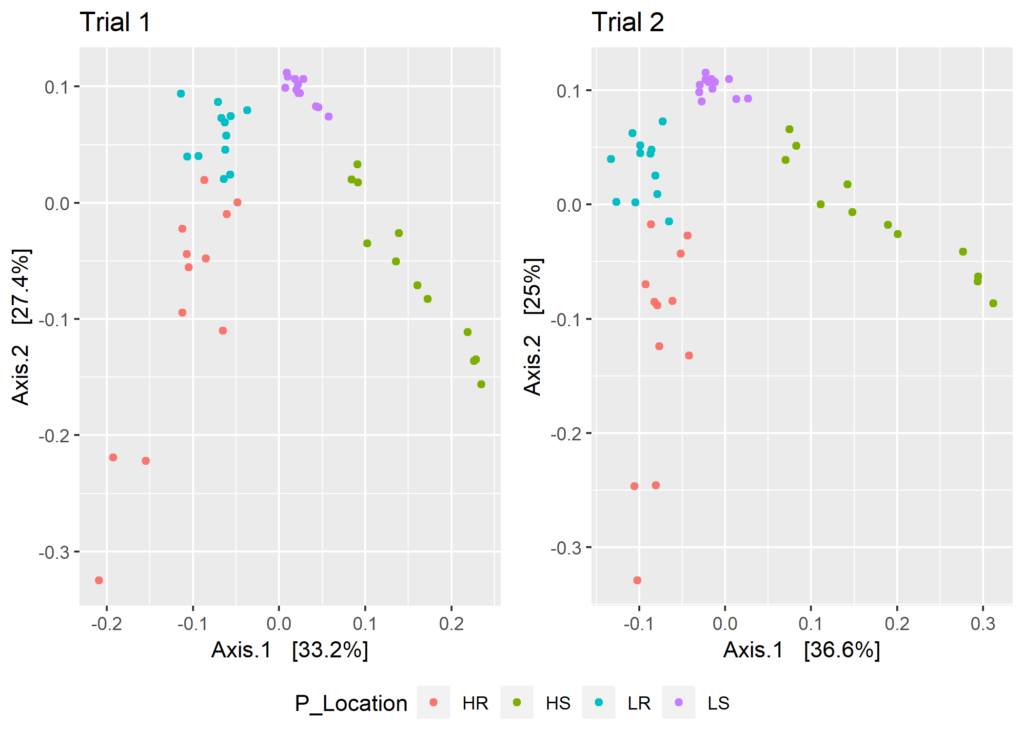

Next I made a Procrustes analysis comparing the two ordinations.

scores.1 <- ord.pf.1$vectors[ , 1:2]
scores.2 <- ord.pf.2$vectors[ , 1:2]
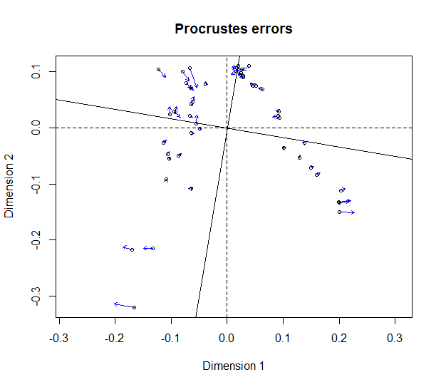
pro <- procrustes(scores.1, scores.2, symmetric = TRUE)
plot(pro)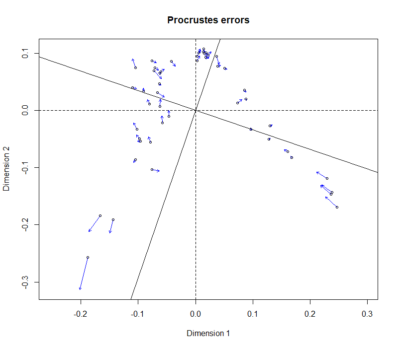

Fig. 2: Plot of Procrustes errors between the two ordinations in Fig. 1.The plot shows relative placement of samples according to the two distance matrices, with the greatest differences in the lower left quadrant.

protest(scores.1, scores.2, permutations = 99999) ##
## Call:  ## protest(X = dw.pd.1, Y = dw.pd.2, permutations = 99999, choices = c(1, 2))
##
## Procrustes Sum of Squares (m12 squared): 0.02374
## Correlation in a symmetric Procrustes rotation: 0.9881
## Significance: 1e-05
##
## Permutation: free
## Number of permutations: 99999

The correlation between the two distance matrices is very high, but not perfect. It is unlikely that such small differences would make a difference in analysis of community differences, by PERMANOVA, for example.

In the discussion mentioned above, Sebastian Schmidt proposed choosing an out group based on the longest tree branch terminating in a tip. His function for finding such an out group is:

pick_new_outgroup <- function(tree.unrooted){
require("magrittr")
require("data.table")
require("ape") # ape::Ntip
# tablify parts of tree that we need.
treeDT <-
     cbind(
         data.table(tree.unrooted$edge),
         data.table(length = tree.unrooted$edge.length)
     )[1:Ntip(tree.unrooted)] %>%
 cbind(data.table(id = tree.unrooted$tip.label))
 # Take the longest terminal branch as outgroup
 new.outgroup <- treeDT[which.max(length)]$id
 return(new.outgroup) }

Applying the function to our data gives us the out group to use to root our tree:

my.tree <- phy_tree(expt)
out.group <- pick_new_outgroup(my.tree)
out.group ## [1] "New.CleanUp.ReferenceOTU8001"

Then we can use this out group to root the tree in expt.

new.tree <- ape::root(my.tree, outgroup=out.group, resolve.root=TRUE)
phy_tree(expt) <- new.tree
phy_tree(expt) ##
## Phylogenetic tree with 31938 tips and 31937 internal nodes.
##
## Tip labels:
## 82502, New.CleanUp.ReferenceOTU38100, 70168, 100112, 113933, 13153, ...
## Node labels:
## Root, , 0.449, 0.000, 0.400, 0.000, ...
##
## Rooted; includes branch lengths.

Now that the tree is rooted, we can calculate the corresponding distance matrix and compare the ordination based on it to one we obtained with phyloseq‘s random root assignment method.

dw.og <- phyloseq::distance(expt, method = "wunifrac")
ord.og<- ordinate(expt, method = "PCoA", distance = dw.og)
plt.3 <- plot_ordination(expt, ord.pf.3, color = "P_Location", title = "By pick_new_outgroup")
plot.3 <- ggarrange(plt.1, plt.3, ncol = 2, legend = "bottom", common.legend = TRUE)
plot.3

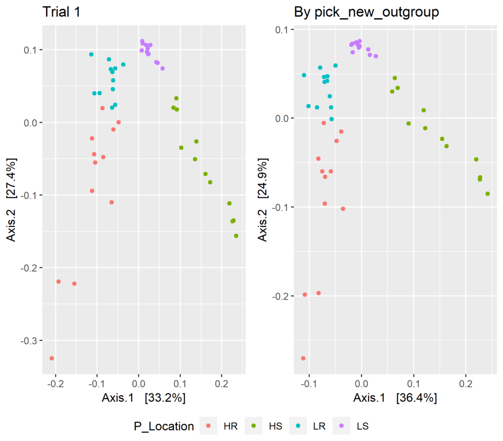
Again, visible inspection reveals some small differences between the ordinations. The overall difference between them can be determined with a Procrustes analysis.

scores.3 <- ord.og$vectors[ , 1:2]
pro <- procrustes(scores.1, scores.3, symmetric = TRUE)
protest(scores.1, scores.3, permutations = 99999) ##
## Call
## protest(X = scores.1, Y = scores.3, permutations = 99999)
## Procrustes Sum of Squares (m12 squared): 0.008256
## Correlation in a symmetric Procrustes rotation: 0.9959
## Significance: 1e-05
## Permutation: free
## Number of permutations: 99999
 plot(pro)

The difference between these two ordinations is certainly no greater than between those obtained with multiple runs taking random root assignments.

Conclusion: I was somewhat surprised that differences between multiple Unifrac calculations with random root assignment could be detected. I had surmised that distances among tree tips would stay the same, and therefore Unifrac distances among samples would stay the same. Perhaps they do, within rounding error.  The differences are certainly too small to impact discrimination of treatments in this data set. Still, I prefer the method based on rooting the tree by the longest branch terminating in a tip because it is not random, and by the function above is easily and quickly done.